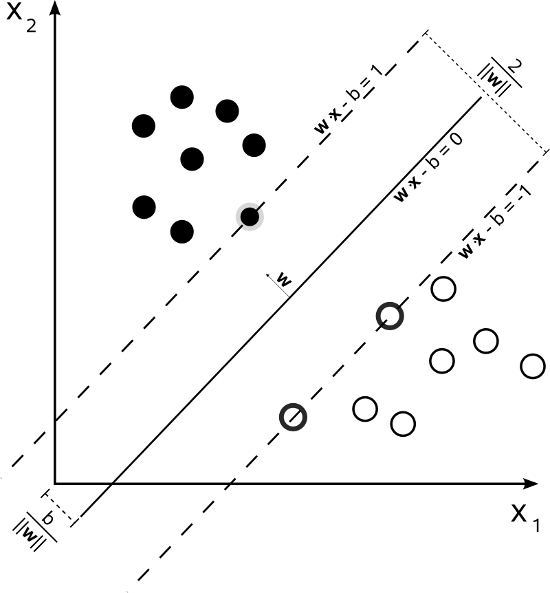
Support Vector Machine(1) - Hard margin maximization

支持向量机

Hyperplane

Consider a two-class separation problem: $$\text{Training set: } T = \left \lbrace (x^{(1)}, y^{(1)}), (x^{(2)}, y^{(2)}) …(x^{(N)}, y^{(N)}) \right \rbrace \\ \text{in which }x^{(i)} \in R^n, y^{(i)} \in \lbrace +1, -1 \rbrace, i=1,2…N$$

Assuming all the samples in the sample space X are linearly separable, we have the hyperplane: $$ w \cdot x + b = 0 \text{, in which }w, b \in R^N$$

Margin

Recall that in the hilbert space, point-plane distance is defined as: $$ \gamma^{(i)} = \left \vert \frac{w}{\Vert w \Vert} \cdot x^{(i)} + \frac{b}{\Vert b \Vert} \right \vert \tag{1.1}$$ Notice that if $x^{(i)}$ is in the same side the normal vector points to, the value would be naturally positive without the absolute function. So if we put the points labelled with +1 in the ‘positive’ space, then $\gamma^{(i)}$ could also be defined as: $$ \gamma^{(i)} = y^{(i)} \left ( \frac{w}{\Vert w \Vert} \cdot x^{(i)} + \frac{b}{\Vert b \Vert} \right ) \tag{1.2}$$

Predicting function

In the other hand, if we have already find the best hyperplane $ w^{*} \cdot x + b^{*} = 0 $ using SVM, given a point $x^{(i)}$, the predicting function would be: $$y^{(i)} = f(x^{(i)}) = sign(w^{*} \cdot x^{(i)} + b^{*}) \tag{1.3}$$

Geometric margin

For a given hyperplane, geometric margin is defined as the minimum distance from the sample point to the plane: $$ \gamma = \min \limits_{i = 1,2…N} \quad \gamma^{(i)} \tag{1.4}$$

Functional margin

Functional margin is defined as: $$ \hat \gamma^{(i)} = y^{(i)} \left ( w \cdot x^{(i)} + {b} \right ) = {\Vert w \Vert} \gamma^{(i)} \tag{1.5}$$ It could be considered as the certainty of the classification. We will soon use it to simplify the maximum problem.

Hard margin maximization

The main purpose of the SVM is to find the hyper plane with the maximum hard margin (geometric margin): $$ \begin{align} & \max \limits_{w,b} \quad \gamma \\ & s.t. \quad y^{(i)} \left ( \frac{w}{\Vert w \Vert} \cdot x^{(i)} + \frac{b}{\Vert b \Vert} \right ) \ge \gamma , \quad i=1,2,…,N \tag{1.6} \end{align}$$

Using functional margin the question could be re-defined as: $$ \begin{align} & \max \limits_{w,b} \quad \frac{\hat \gamma}{\Vert w \Vert} \\ & s.t. \quad y^{(i)} \left ( w \cdot x^{(i)} + {b} \right ) \ge \hat \gamma , \quad i=1,2,…,N \end{align} \tag{1.7}$$

Notice that for a given hyper plane, $\Vert w \Vert$ and $\Vert b \Vert$ could vary since $w$ and $b$ could stretch in the same direction arbitrarily without changing the hyper plane. To constrain this, we confine $\hat\gamma = 1$(this is an important step to constrain $\Vert w \Vert$ into a fixed scale), the problem finally becomes: $$ \begin{align} & \min \limits_{w,b} \quad \frac{1}{2} {\Vert w \Vert}^2 \\ & s.t. \quad y^{(i)} \left ( w \cdot x^{(i)} + {b} \right ) - 1 \ge 0, \quad i=1,2,…,N \end{align} \tag{1.8}$$

$\min \limits_{w,b} \frac{1}{2} {\Vert w \Vert}^2$ equals $ \max \limits_{w,b} \frac{1}{\Vert w \Vert} $, which is the original problem.

Soft margin maximization

If the samples is not linearly separable, to solve this problem, set a loose vector $\xi \in R^n$ for each sample, then the restriction in (1.8) becomes: $$ y^{(i)} \left ( w \cdot x^{(i)} + {b} \right ) + \xi_i - 1 \ge 0 \tag{1.9}$$ For each sample, pay a cost $\xi_i$ in the target function: $$ \frac{1}{2} {\Vert w \Vert}^2 + C \sum\limits_{i=1}^{N}\xi_i \tag{1.10}$$ $C$ is called the penalty parameter, the larger $C$ means a more strict SVM classifier.

How to solve the margin maximization problem? (to be continued)

Support Vector

Maximum-margin hyperplane and margins for an SVM trained with samples from two classes. Samples on the margin are called the support vectors.